In this post, a simple statistical inference task of a modeling a coin flip shall be our vehicle to introduce important statistical concepts. These concepts will become central to our study in Singular Learning theory. We shall show our calculations with excruciating details in hope that such simple case will be instructive and serve to define the limits of our tools in extracting exact results.

Post summary:

To model the outcome of a coin flip, we introduce a general way to do statistical inference by constructing a parameterised model - a family of probability distributions, each a possible approximation to the process that generates the coin flips. We introduce the likelihood function . It gives the probability of observing the given data set assuming they are generated by the model at a specified parameter.

We introduce a popular statistical estimation method, the Maximum Likelihood method, to estimate the outcome of a coin flip. With this method, the likelihood function is treated as an objective function to be maximised and the model at the maximum is used to approximate the truth. We point out that the result of such an inference procedure is itself random. Specifically, it depends on the random sampling that generates the data set. It is the role of a statistical learning theory to clarify if a certain statistical estimation procedure is to be employed

• What is the expected performance given subject to the randomness of training samples?
• For what class of true data generating process would the procedure approximate well?

Using the normal approximation to the binomial distribution, we shall see that the maximum likelihood estimator for the coin flip model is asymptotically normal and asymptotically efficient two desirable properties that is the hallmark of regular model but are absent in singular models.

• The Situation, The Dataset
• Statistical Inference
  • Models
  • Learning and Inference
• The Adventure of Maximum Likelihood Estimation
  • Empirical Log Loss and Log Likelihood Ratio
  • Finally Some Calculations
  • So how did we do?
• A Broader Theory of MLE and Fisher Information
• Role of Statistical Learning Theory

The Situation, The Dataset

Suppose there is a coin-flipping demon on the other side of a door. He offers us a deal. We can bet a number of years of our remaining life. If his next coin flip turns out to be head, he will pay us double what we bet. Otherwise, he keeps the bet. Rather uncharacteristicallyor maybe it’s just a deception, he offers to first perform $N$ flips and let us look at the results. We shall call this set of observations

\[D_N = \set{X_1, X_2, \dots, X_N}, \quad X_i \in \set{H, T}\]

our dataset or training samples .

As a pure utilitarian, we decide to not run. Which means we better have a really good estimate of the probability $\hat{p}$ of the next flip turning out heads since most sound betting strategy relies on it. For instance, the Kelly’s criterion gives the optimal fraction of our life in this situation as $2 \hat{p} - 1$ .

Statistical Inference

Models

So we are in a situation where we are given a training set, $D_N$, of previous coin flips and our task is to estimate the probability $\hat{p}$ that the next flip comes up head.

Let $h$ denote the number of heads in the dataset $D_N$ and $t = N - h$ the number of tails.

Model 0. We can simply guess that it's a fair coin so that $\hat{p} = 1/2$. This is a not a good inference method not less because a demon wouldn't be fair. There is no learning involved at all. We ignored the dataset, which should be a valuable resource in dealing with a demon. Even in this case, we are still left with questions like when exactly is this method badjust so that no one will come and say "I told you so" when the demon actually uses a fair coin and how to quantify exactly how bad the method is.

Model 1. We can instead construct a family of hypothesis, parameterised by $w \in [0, 1]$. Each $w$ represent a guess that the probability of landing heads $=w$. We say that we are defining a model $$ p(X \mid w) = \begin{cases} w, & X = H \\ 1 - w, & X = T \end{cases} $$ with parameter $w$ taking value in the parameter space $W = [0, 1]$. We can now reason as follow:
If the probability of landing heads were to be $w$, then the probability that the dataset $D_N$ that we observed get generated is $$ p(D_N \mid w) = \prod_{i = 1}^N p(X_i \mid w) = w^h (1 - w)^t. $$

Notice that we are assuming that, on the other side of the door, the demon is consistently throwing the same coin in the same way, so that we get a constant probability of landing heads. We call this true probability of landing heads the true parameter $w_0$. This means that each $X_i$ follows an identical distribution, $p(H) = w_0$, and that each observation is independent of all others. Together, this is the common independent and identically distributed (i.i.d) assumption that allows us to factorise $p(D_N\mid w)$ as we did aboveWe could stipulate additionally that the order of $X_i$ doesn't matter, introducing a factor of $\binom{N}{h}$ making the above the binomial distribution. But we omit this for exposition uniformity. The binomial coefficient will be reintroduced whenever we sum over these sequences anyway. . We call the probability of observing a given dataset for a given parameter the likelihood function $$l_N(w) = p(D_N \mid w)$$ which, to emphasise, is a function of paramter $w$ with the dataset $D_N$ fixed.

Model 2. But the demon could be more ... demonic. Every time he does a flip, he could've been choosing one of two coins at random from a box, only one of which is a fair coin. We can introduce another parameter $s \in [0,1]$ for representing the probability that the fair coin is chosen and $w \in [0, 1]$ represent the bias - probability of landing heads - for the other coin. We have now a two dimensionalbut still compact paramter space $(s, w) \in [0, 1]^2$. The hypothesis at each parameter is given by $$ \begin{align*} p(H \mid s, w) &= \frac{1}{2}s + w (1 -s) \\ p(T \mid s, w) &= \frac{1}{2}s + (1 - w) (1 - s) \end{align*} $$ and the likelihood function becomes $$ l_N(w) = \prod_{i = 1}^Np(X_i \mid s, w) = \brac{\frac{1}{2}s + w (1 -s)}^h \brac{\frac{1}{2}s + (1 - w)(1 -s)}^t $$ which again uses the i.i.d assumption.

Learning and Inference

We could continue to imagine more and more demonic opponent on the other side, but we should first see what can the models do for us.

We can continue the reasoning with likelihood function as follow:

We now have $l_N$ giving us the probability of observing $D_N$ for specific parameter.
Surely the most likely $w$ is the one that give the highest probability for the observed data? this reminds me a little of the antropic principle. Hence we should set the estimate $\hat{p}$ to be the parameter $w$ that maximises $l_N(w)$.

This gives us the statistical inference method known as Maximum Likelihood Estimate (MLE), i.e. find the single parameter this makes it a point estimate. $w$ that maximises the likelihood function.

This is a natural line of reasoningthere was a time when I was only taught this method of statistical estimation and think this is the only way., and indeed it is in some sense the correct method for this situation.

However, MLE assumed quite a few things.

• MLE says “surely another coin with a different probability of landing heads would produce quite different looking observations $D_N$?”. Well, not really. What if there is only one observation $N = 1$? Let’s say $D_1 = \set{H}$. Surely a whole range of $w$ could’ve plausibly generated itas we shall see, the MLE answer in this case would be at the boundary of $[0, 1]$, $\hat{p} = 1$ which, at least to me, doesn’t seem to be a well-justified answer.?
• “Ah, but if $N$ is truly huge, small difference in $w$ will result in very different $D_N$”, says MLE. We shall see that this is indeed true. As the number of observations grow, it becomes asymptotically impossible for another parameter but the true one to generate the sequence of coin flips observed.
• BUT, that is only true if we made the assumption that the true parameter is contained in the model! This is the realisability assumption. For instance, if the demon is really following the coin flipping recipe laid out in model 2 above, then maximising the likelihood function of model 1 how much worse is model 0?wouldn’t give us accurate answer, not even asymptotically.
• MLE doesn’t provide the answer to the quenstion “what is the most likely parameter given the observation” $= p(w \mid D_N)$, which is a distinct question to “what is the most likely observation given the parameter” $= p(D_N \mid w)$.

The Adventure of Maximum Likelihood Estimation

Despite the above misgiving, we shall push through with MLE of model 1. We shall have explicit computation and introduce several important statistical concepts along the way. We shall see in what sense is MLE a good estimator in this case and what could go wrong in other situations where we might like to use the same procedure.

We shall also make the realisability assumption where the demon’s coin flip follows the following true distribution

\[\begin{align*} q(H) &= w_0 \\ q(T) &= (1 - w_0) \end{align*}\]

for some true paramter $w_0 \in [0, 1]$. Meaning $q(x) = p(x \mid w_0)$.

Empirical Log Loss and Log Likelihood Ratio

We wish to set $\hat{p} =$ the maximum of the likelihood function

\[l_N(w) = w^h (1 - w)^t.\]

If $N$ is a large number, the above expression produces really small numbers which can be numerically challenging to handle. We usually do a monotonic hence doesn’t change any extrema of the function transform by taking its logarithm, which also happily simplifies several calculations. In fact, we shall introduce the empirical log loss function

\[L_N(w) = -\frac{1}{N} \log p(D_N \mid w) = -\frac{1}{N} \sum_{i = 1}^N \log p(X_i \mid w)\]

which we shall aim to minimisehence the usage of the term “loss”.. In our case, we get

\[L_N(w) = \frac{1}{N} \brac{\sum_{X_i = H} \log w + \sum_{X_i = T} \log (1 - w)} = \frac{1}{N} \sqbrac{h \log w + t \log (1 - w)}\]

Below is a little tangent justifying the introduction of this quantity and its connection to the log likelihood ratio function which will be an important information theoretic quantity for our study.

Connection to log likelihood ratio

The Shanon entropy of the true distribution is given by $$ S(q) = -\E_q(\log q(X)) = -q(H)\log q(H) + -q(T) \log q(T) $$ which can be approximated by the empirical entropy using the observation from the data set $D_N$ $$ S_N(q) = -\frac{1}{N} \sum_{i = 1}^N \log q(X_i). $$ Adding this quantity to the empirical log loss function we get the empirical log likelihood ratio $$ K_N(w) = \frac{1}{N} \sum_{i = 1}^N \log \frac{q(X_i)}{p(X_i \mid w)} = -\frac{1}{N} \sum_{i = 1}^N \log p(X_i \mid w) + \frac{1}{N} \sum_{i = 1}^N \log q(X_i) = L_N(w) - S_N(q) $$ which is the empirical estimate to the central object of study, the expected log likelihood rato better known as the Kullback-Leibler divergence of the model at $w$ to the true distribution $$ K(w) = D_{KL}(q(x) \mid \mid p(x \mid w)) = \E_X\sqbrac{\log \frac{q(X)}{p(X \mid w)}}. $$ We note that minimising $K_N(w)$ is equivalent to minimising $L_N(w)$ since they differ by an additive constant that is independent of $w$.

Finally Some Calculations

Since our objective function $L_N(w)$ is a differentiable function, we shall use the stationary point criterion for finding local minima.

So, we find that maximimum likelihood estimate is given by

\[\hat{p} = \hat{w} = \frac{h}{N}.\]

It’s important to emphasise again that $h$ in the expression above is the number of heads in the given data set $D_N$, it depends on the given set of observations so is itself a random variable!indeed, even functions we defined like $l_N(w)$, $L_N(w)$, $K_N(w)$ are all random variables, they just take values in the space of functions. This is why proper investigation into their behaviour in statistical learning theory requires functional analysis.

So how did we do?

Though we now have our estimate, there is still a concern that we might have gotten an atypical data set which makes our guess wildly inaccurate. We need some way to quantify the uncertainty of our $\hat{w} = h / N$ estimate. Fortunately, we can do some exact calculation in this case.

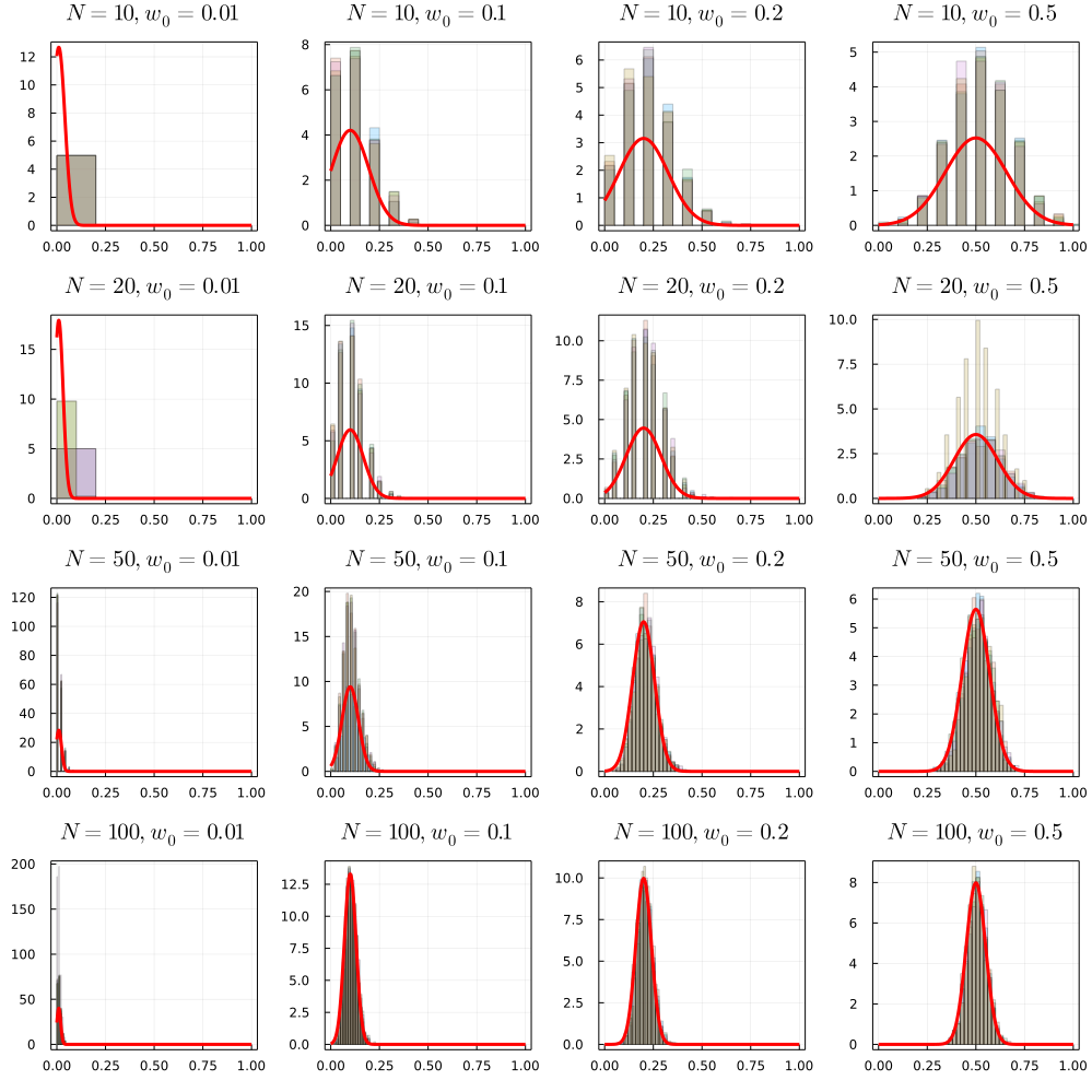
The asymptotic normality $\hat{w} \to N(Nw_0, Nw_0 (1 - w_0))$ uses the normal approximation to binomial distribution. can be proven by apply the Central Limit Theorem to sums of Bernoulli random variables or directly use a classic result of de Moivre-Laplace.

The array of plots below shows the normal density superimposed on histograms of $\hat{w}$ for different values of $N$ and $w_0$. Observe that the normal approximation works better for large values of $N$ and away from pathological values of $w_0 = 0, 1$. The closer the true parameter $w_0$ is to the boundary, the large the data set needs to be for the normal distribution to correctly approximate the density away from the meanImagine $w_0$ being close to the boundary, then when $N$ is small the variance $w_0(1 - w_0) / N$ is large, which makes a large portion of the normal density extends in to the “imppossible” region $ \hat{w} \not\in [0, 1]$. .

A Broader Theory of MLE and Fisher Information

Having been forced by the demon to go through these exercises in statistical inference we noticed a few things about MLE for model 1:

• The maximum likelihood parameter exist and is unique, even when it turns out to be at the boundary $\hat{w} = 0, 1$.
• It is an unbiased estimator, meaning the expected MLE prediction gives the true paramter (again, assuming realisability.)
• It is asymptotically normal, meaning as the number of observations $N \to \infty$, the distribution of $\hat{w}$ approaches that of the normal distribution.
• It turns out that the form the of asymptotic normal distribution implies that $\hat{w}$ achieves asymptotic efficiency , meaning it achieves the lowest variance possible for any unbiased estimator as prescribed by the Cramer-Rao inequality.

Before we state the Cramer-Rao bound, we need a few preliminaries. It turns out that the above is actually true for MLE of a large class of models $p(x \mid w)$ modeling some true distribution $q(x)$ satisfying some regularity conditions which turns out to be far too strong for general statistical learning theory. Hence the need to study “Singular Models”. .

Even with slightly more complicated models, it is unlikely that we will have the luxury of computing the estimator distribution exactly as we did in this simple case. However, taking limits ($N \to \infty$) is always a good way to wash away the details.

Perhaps the most famous among the tools for washing away details is the Central Limit Theorem

So, if somehow our estimators are sums of increasingly numerous i.i.d. random variables, we have asymptotic normality. Just like in the case of the coin flip where the number of heads $h$ is given by sums of i.i.d. random variables $\sim Bernoulli(w_0)$. We might not have that in general. However, it turns out that the spread of MLE estimator is related to the following object.

In the 1D case, this reduces to a scalar function

\[I(w) = \V_{X \sim p(x \mid w)}(\frac{\partial}{\partial w}\log p(X \mid w)) = \int \brac{\frac{\partial}{\partial w}\log p(x \mid w)}^2 p(x \mid w) dx.\]

We interpret this as answering the following question:

If the data were sampled from the distribution at $w$, $X_i \sim p(x \mid w)$, what is the variance of the $\frac{d}{dw} \log p(x \mid w)$, the log-likelihood ratio.

Recall that we use the condition that $\frac{d}{dw} \log p(x \mid w)$ to find (local) maximum of the likelihood function which we then take as our estimate of the true parameter. So, informally, $I(w)$ is related to the spread of our MLE prediction.

Computing this quantity for our coin toss model,

we get

\[I(w) = \frac{1}{w(1 - w)}.\]

The lemma proven above shows that $I(w) = \E_{X \sim p(x \mid w)} \sqbrac{-\partial^2_w \log p(x \mid w)}$. This gives another intuition of what $I(w)$ measures:

If the data were sampled from the distribution at $w$, what is the expected curvature of the log-likelihood near $w$?
Said another way: If the true parameter $w_0$ were to be at $w$, what is the expected curvature of the log-likelihood near the true parameter?

From the calculation, at the true parameter $I(w_0) = (n \sigma^2)^{-1}$ where $\sigma^2 = w_0(1 - w_0) / N$ is the variance of $\hat{w}$ computed before. This relationship between estimator variance and Fisher information is not a coincidence. It is evidence that MLE for our model above is asymptotically efficient. This means that the $\sigma^2$ is the tightest asymptotic spread of our estimator possible. Put another way, our MLE achieves the Cramer-Rao lower bound stated below.

The theorem says that the Fisher information matrix give the highest precision or the lowest possible variance precision $= 1 / $ variance any unbiased estimator can achieve. In fact, this is more general than just the MLE for our simple coin toss case.

Some regularity conditions:

It is rather complex to carefully state the regularity conditions here. For rigorous discussions, see (Lehmann, 2005, chapter 12). But the conditions frequently involves

• $W$ is an open subset.
• The model is identifiable. Meaning distinct parameters gives distinct probability density.
• The density $p(x \mid w)$ for any $w$ has common support.
• $p(x \mid w)$ is thrice continuously differentiable with respect to $w$.
• The model has positive definite Fisher information matrix.

Also, notice that the lower bound does not apply when $I(w) = 0$ such as when $w = 0, 1$ in our coin toss model and more generally when $I_{ij}(w)$ is not an invertible matrix.

Role of Statistical Learning Theory

The role of statistical learning theory is to clarify the performance of procedures like MLE we used above. What if it is not realisable? This is a rather common case for modeling complex processes. What if the true parameter is at a singularity of the model? Nearby points are affected as well. What happen when $N$ is small?

Lehmann, E. L., and Joseph P. Romano. 2005. Testing Statistical Hypotheses. Springer, New York, NY.